HF Near Vertical Incidence Skywave (NVIS) Frequency Band Selection

Near Vertical Incidence Skywave (NVIS) Propagation

NVIS propagation is used to fill in between the distance that is normally covered by ground wave and the first hop for low angle of radiation long distance communication. This typically falls between 50 miles and 600 miles.

NVIS is often compared to pointing a shower head straight up at the ceiling and having the water droplets fall everywhere. Counter to most HF antenna installations, NVIS requires a high angle of radiation. This is achieved by installing the antenna at a low height, usually no higher than 1/8 wavelength. Lower antenna heights result in only a slight reduction in received signals and it is not atypical for a portable installation to have the antenna installed just a few feet above the ground.

NVIS does not require a high transmit power level. Power levels of 25 watts are quite effective in maintaining good quality HF communications.

NVIS requires using a frequency that is below the Critical Frequency, the highest frequency at which NVIS communications can operate at, but above the frequency at which the D-Layer absorption results in excessive attenuation, or the Lowest Usable Frequency (LUF). NVIS communications is not possible below the LUF or above the Critical Frequency. Use of frequencies below the LUF or above the Critical Frequency will result in a loss of NVIS communications.

For all practical purposes, NVIS communications at Idaho latitudes rarely are usable at frequencies above 13 MHz as the Critical Frequency rarely climbs above this level.

NVIS HF Propagation is in daily use by United States Military Forces and government emergency agencies at all levels of government on a daily basis. The reason is that it works very reliably.

NVIS Critical Role

NVIS is typically used for communication ranges of from 50 to 600 miles. When topographical features, such as mountainous terrain, are involved, the typical ground wave distance of 50 miles can be reduced to very short distances. Ground wave distances can also vary in distance where the take off angle of radiation goes over the top of the target station or where terrain obstructs the radio wave from reaching the target station. Ground wave may be reduced to even a few miles.

Between the D-Layer absorption frequency (LUF) and the Critical Frequency, reliable NVIS communications can be had and will fill in the distances between ground wave and long hop propagation. NVIS capabilities present the best option for communications that span between ground-wave and approximately 600 miles.

Automatic Link Establishment (ALE)

Automatic Link Establishment implements a combination of control of radio frequency, multi-frequency shift keying and digital sounding protocols to determine the limits of the D-Layer absorption frequency (LUF), critical frequency and maximum usable frequency based on a periodic process of trial and succeed/fail. When an NVIS antenna configuration is in place, and distances fall between ground-wave and long-hop propagation, then the successful trials span between the LUF and Critical Frequency and indicates those frequencies at which NVIS communications is possible.

Although ALE radios are available for amateur radio use, or PC-ALE is available as an option to implement ALE through serial interface control of the radio, most amateurs do not have ALE capability. The PC-ALE option may not be viable for radios with relay band switching as the sounding process implements scanning across multiple bands, resulting in relay activity as the bands are traversed. This could result in radio reliability issues. PC-ALE may only be a viable option for radios that implement diode switching of filter sections and where relays are not used in band switching activity.

Further NVIS ALE for the amateur radio operator is generally limited by propagation conditions to the the following bands:

• Voice Communications

  • 75m

  • 60m

  • 40m

• Data Communications

  • 80m

  • 60m

  • 40m

  • 30m

ALE has the potential to help resolve issues of HF frequency planning. However, ALE radios are not readily available in the amateur radio marketplace and the option for computer controlled ALE alternatives exclude Linux and Mac OS X operating platforms under the native operating system. PC-ALE can be made to operate on Linux or Mac OS X under the Windows operating system while running Windows in a virtual machine (such as VM Ware - Fusion).

Fortunately, with the availability of propagation data on the internet, there are viable alternatives to ALE in determining usable HF frequencies.

Ionosonde Data Interpretation

Many HF operators hear a signal periodically sweep through the band. This is often mistaken for a station transmitting a carrier while sweeping the VFO. In reality, this is an ionosonde. An ionosonde makes transmissions while sweeping across the spectrum to determine the D-Layer absorption frequency (LUF), Critical Frequency and Maximum Usable Frequency.

Ionosonde data is charted from ionosonde stations world-wide. The closest ionosonde station for Idaho is located at Boulder, Colorado. It should be noted that, due to differences in latitude and longitude, propagation trends in Idaho will lag behind trends indicated by the Boulder ionosonde.

Ionosonde data from many stations is translated from raw tables of data into charts that are usable for interpretation by the average amateur radio operator. Further, some stations also chart the trend of the Critical Frequency, with plots representing the current day, previous day and previous five days.

The following image depicts an ionogram.

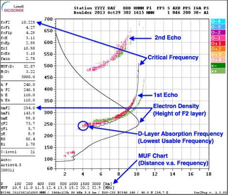
The Critical Frequency, the highest frequency at which NVIS propagation can be used, is depicted as the foF2 frequency on the chart at the left of the graph and as the upper frequency limit of the first echo sounding curve.

The D-Layer absorption frequency, or Lowest Usable Frequency (LUF), is shown as the lower frequency limit of the first echo sounding curve.

The MUF chart at the bottom shows distances, in kilometers, versus the maximum usable frequency appropriate for the distance. Note that a conversion factor must be applied to determine the MUF for distances in miles (i.e. distance in kilometers X 0.62137119 = distance in miles).

An additional resource, available from ionosonde reporting stations, shows the Critical Frequency trend for the current day and the previous five days, as shown in the following graph:

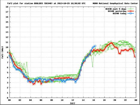
The Critical Frequency trend is simply the foF2 data, derived from ionosonde data, and plotted over time. The blue line represents the current day.

The graph of the Critical Frequency trend provides a quick and easy method of determining the proper NVIS frequency by picking the band closest to, but not exceeding the Critical Frequency.

The two charts above were obtained on the 29th of October, 2013. The ionogram was obtained at 1615 UTC (i.e. 1015 mountain time) while the Critical Frequency Trend chart was obtained at 1630 UTC (i.e. 1030 mountain time). From these two charts, it can be seen that the optimum NVIS frequency falls between the D-Layer absorption frequency of 4.00 MHz and the foF2 frequency of 10.225 MHz, indicating that the 40-meter amateur band is the optimal band for NVIS communications at 1630 UTC (1030 mountain) on the 29th of October.

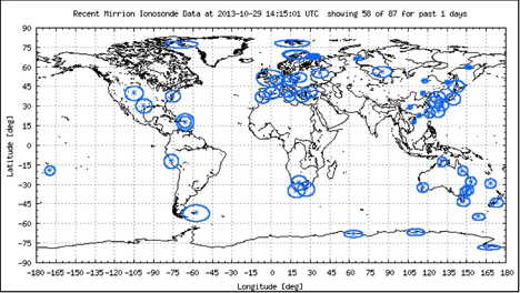
In addition to the ionogram and critical frequency trend, the Australian government publishes a real-time global map of the foF2 critical frequency, as depicted below:

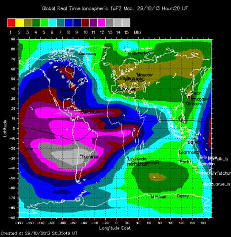
This map uses color coding to indicate the critical frequencies across the globe. The map is useful in determining the maximum frequency that can be used for NVIS communications, however, the D-Layer absorption frequency, which is not depicted on the map, must be considered in order to determine the minimum frequency that is usable for NVIS or long-hop communications.

NOTE: A current depiction of the above propagation map can be found on the Propagation page found under the Resources menu on this site.

NOTE: Using the above map resource, you can perform an approximate short term prediction of what conditions may occur in the near future. Each 15° of longitude represents one-hour. By skewing to the right from your operation location by 15° of longitude, you can approximate the conditions you will experience in 1-hour. Use 30° for 2-hours, 45° for 3-hours, etc. Be aware that the size and colors of the blobs that represent the foF2 NVIS Critical Frequency can change rapidly. Any future propagation predictions are only an approximation, and the further forward in time for the prediction, the higher the probability that the prediction will not be accurate.

NOTE: Where the above map indicates the foF2 NVIS Critical Frequency, the relationship between the foF2 frequency and the Maximum Usable Frequency (MUF) is approximately 1:3. Multiplying the foF2 critical frequency by 3 approximates the MUF. Because of the relationship between foF2 and MUF, the above map can also be used to determine frequencies for use with skywave propagation. The following color chart, which is applicable to the foF2 critical frequency map above, is adjusted to indicate the MUF.

The following animated map shows how the colored frequency zones move from east to west. The animation will pause for 2-seconds on the last frame before looping.

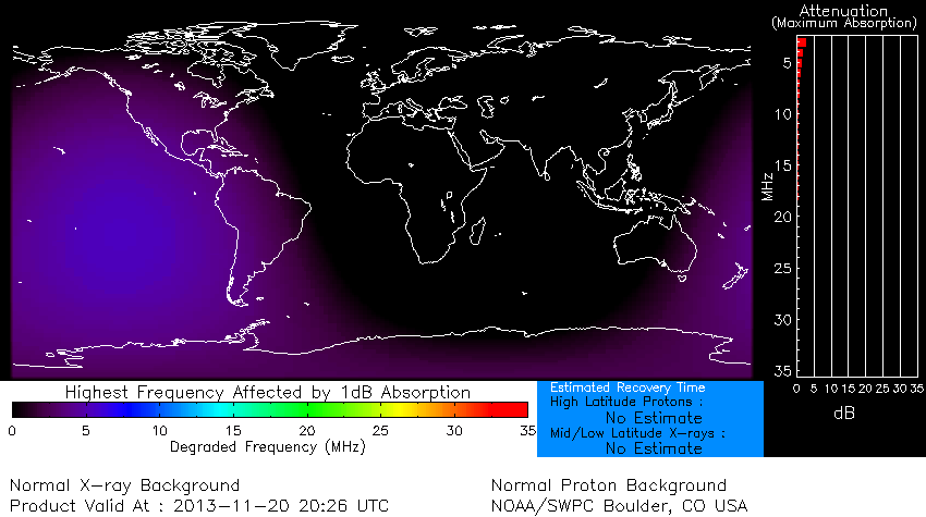
The National Oceanic & Atmospheric Administration (NOAA) publishes real-time prediction of the D-Layer absorption frequency, which is depicted worldwide on a map. The color shading on the map indicates the minimum frequency that can be used for either NVIS or long hop propagation.

Determining HF NVIS Operating Frequencies

Determine the communications distances for all stations to be contacted and select a frequency that falls above the D-Layer absorption frequency, as indicated by the lower frequency limit of the 1st echo curve, and below the Critical Frequency (i.e. foF2 frequency) from the chart at the top left of the ionogram.

Determining HF Long-Hop Operating Frequencies

Determine the communications distances for all stations to be contacted and select a frequency that falls below the MUF for the specified distance as indicated in the MUF chart.

Where To Find Ionosonde Data

Propagation information from multiple web pages is pulled together into a single web page by clicking here or by selecting the Propagation and Weather page that is available under the Resources menu above.

D-Layer Absorption Frequency Trend

The D-Layer absorption frequency trend does not appear to be plotted. The amateur radio operator can plot the D-Layer absorption frequency trend from available ionogram data, or can simply observe the critical frequency directly from the current ionogram.

When plotted, the D-Layer absorption frequency trend gives good insight into the Lowest Usable Frequency (LUF) as the day progresses:

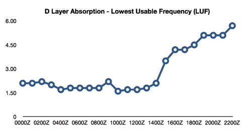
The plot above shows the 75m band becoming unusable for NVIS propagation between 1400 UTC (1000 Mountain) and 1500 UTC (1100 Mountain). This is not atypical of observed daily conditions on 75m.

VOACAP Propagation Predictio

Although VOACAP propagation prediction appears to be accurate for long hop communications, it does not appear to be accurate for NVIS and ground-wave propagation prediction. VOACAP appears to be overly aggressive in predicting propagation toward the short end of NVIS communications ranges, as if there may be reliance on ground-wave propagation that simply is not realized with mountainous terrain.

Conclusion and Recommendations

Since the D-Layer absorption frequency (LUF) and Critical Frequency tend to move throughout the day, and vary with space weather, any operational planning should include contingencies for variations in propagation conditions.

The following table provides recommendations for NVIS communications:

Determining An NVIS Frequency Band To Use
D-Layer Absorption Frequency (LUF) MHz	Critical Frequency (foF2) MHz	Recommended Operating Band
3.5>LUF	4.0 < foF2 AND foF2 < 4.0	80-meters / 75-meters
4.0 < LUF AND LUF < 5.0	5.3 < foF2 AND foF2 < 7.0	60-meters
5.2 < LUF AND LUF < 7.0	7.3 < foF2 AND foF2 < 10.0	40-meters
7.3 < LUF AND LUF < 10.0	10.2 < foF2 AND foF2 < 14.0	30-meters
10.2 < LUF AND LUF < 14.0	14.5 < foF2 AND foF2 < 18.0	20-meters

The daily progression of the D-Layer absorption frequency, critical frequency and maximum usable frequency is fairly consistent, baring any perturbation by space weather. D-Layer absorption usually renders 80m/75m unusable for NVIS by mid morning, with conditions shifting to the 60m band. By mid day, conditions shift from 60m to 40m. The cycle reverses itself as evening approaches and passes.

For NVIS propagation, always choose an operating frequency that is between the D-Layer absorption frequency (LUF) and the Critical Frequency.